Regional model ICON-D2 The DWD's ICON-D2 model is a forecast model which is operated for the very-short range up to +27 hours (+45 hours for the 03 UTC run). Due to its fine mesh size, the ICON-D2 especially provides for improved forecasts of hazardous weather conditions, e.g. weather situations with high-level moisture convection (super and multi-cell thunderstorms, squall lines, mesoscale convective complexes) and weather events that are influenced by fine-scale topographic effects (ground fog, Föhn winds, intense downslope winds, flash floods). The model area of ICON-D2 covers the whole German territory, Benelux, Switzerland, Austria and parts of the other neighbouring countries at a horizontal resolution of 2.2 km. In the vertical, the model defines 65 atmosphere levels. The fairly short forecast periods make perfect sense because of the purpose of ICON-D2 (and its small model area). Based on model runs at 00, 06, 09, 12, 15, 18 and 21 UTC, ICON-D2 provides new 27-hour forecasts every 3 hours. The model run at 03 UTC even covers a forecast period of 45 hours. The ICON-D2 forecast data for each weather element are made available in standard packages at our free DWD Open Data Server, both on a rotated grid and on a regular grid. Regional ensemble forecast model ICON-D2 EPS The ensemble forecasting system ICON-D2 EPS is based on the DWD's numerical weather forecast model ICON-D2 and currently includes 20 ensemble members. All ensemble members are calculated at the same horizontal grid spacing as the operational configuration of ICON-D2 (2.2 km). Like ICON-D2, the ICON-D2 EPS ensemble system provides forecasts up to +27 hours for the same model area (up to +45 hours based on the 03 UTC run). For generating the ensemble members, some of the features of the forecasting system are changed. The method currently used to generate the ensemble members involves varying the - lateral boundary conditions - initial state - soil moisture - and model physics. For varying the lateral boundary conditions and the initial state, forecasts from various global models are used. The ICON-D2 EPS is provided on the DWD Open Data Server in the native triangular grid. Note: All previously COSMO-D2 based aviation weather products have been migrated to ICON-D2 on 10.02.2021. However, the familiar design of these products remains unchanged.

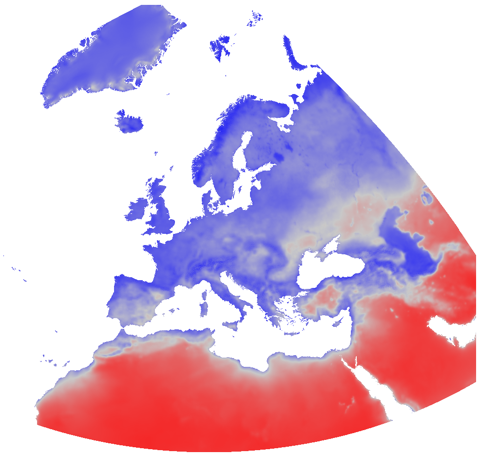
Overview: ERA5-Land is a reanalysis dataset providing a consistent view of the evolution of land variables over several decades at an enhanced resolution compared to ERA5. ERA5-Land has been produced by replaying the land component of the ECMWF ERA5 climate reanalysis. Reanalysis combines model data with observations from across the world into a globally complete and consistent dataset using the laws of physics. Reanalysis produces data that goes several decades back in time, providing an accurate description of the climate of the past. Processing steps: The original hourly ERA5-Land air temperature 2 m above ground and dewpoint temperature 2 m data has been spatially enhanced from 0.1 degree to 30 arc seconds (approx. 1000 m) spatial resolution by image fusion with CHELSA data (V1.2) (https://chelsa-climate.org/). For each day we used the corresponding monthly long-term average of CHELSA. The aim was to use the fine spatial detail of CHELSA and at the same time preserve the general regional pattern and fine temporal detail of ERA5-Land. The steps included aggregation and enhancement, specifically: 1. spatially aggregate CHELSA to the resolution of ERA5-Land 2. calculate difference of ERA5-Land - aggregated CHELSA 3. interpolate differences with a Gaussian filter to 30 arc seconds. 4. add the interpolated differences to CHELSA Subsequently, the temperature time series have been aggregated on a daily basis. From these, daily relative humidity has been calculated for the time period 01/2000 - 07/2021. Relative humidity (rh2m) has been calculated from air temperature 2 m above ground (Ta) and dewpoint temperature 2 m above ground (Td) using the formula for saturated water pressure from Wright (1997): maximum water pressure = 611.21 * exp(17.502 * Ta / (240.97 + Ta)) actual water pressure = 611.21 * exp(17.502 * Td / (240.97 + Td)) relative humidity = actual water pressure / maximum water pressure Data provided is the daily averages of relative humidity. Resultant values have been converted to represent percent * 10, thus covering a theoretical range of [0, 1000]. The data have been reprojected to EU LAEA. File naming scheme (YYYY = year; MM = month; DD = day): ERA5_land_rh2m_avg_daily_YYYYMMDD.tif Projection + EPSG code: EU LAEA (EPSG: 3035) Spatial extent: north: 6874000 south: -485000 west: 869000 east: 8712000 Spatial resolution: 1000 m Temporal resolution: Daily Pixel values: Percent * 10 (scaled to Integer; example: value 738 = 73.8 %) Software used: GDAL 3.2.2 and GRASS GIS 8.0.0 Original ERA5-Land dataset license: https://apps.ecmwf.int/datasets/licences/copernicus/ CHELSA climatologies (V1.2): Data used: Karger D.N., Conrad, O., Böhner, J., Kawohl, T., Kreft, H., Soria-Auza, R.W., Zimmermann, N.E, Linder, H.P., Kessler, M. (2018): Data from: Climatologies at high resolution for the earth's land surface areas. Dryad digital repository. http://dx.doi.org/doi:10.5061/dryad.kd1d4 Original peer-reviewed publication: Karger, D.N., Conrad, O., Böhner, J., Kawohl, T., Kreft, H., Soria-Auza, R.W., Zimmermann, N.E., Linder, P., Kessler, M. (2017): Climatologies at high resolution for the Earth land surface areas. Scientific Data. 4 170122. https://doi.org/10.1038/sdata.2017.122 Processed by: mundialis GmbH & Co. KG, Germany (https://www.mundialis.de/) Reference: Wright, J.M. (1997): Federal meteorological handbook no. 3 (FCM-H3-1997). Office of Federal Coordinator for Meteorological Services and Supporting Research. Washington, DC Acknowledgements: This study was partially funded by EU grant 874850 MOOD. The contents of this publication are the sole responsibility of the authors and don't necessarily reflect the views of the European Commission.

The Copernicus DEM is a Digital Surface Model (DSM) which represents the surface of the Earth including buildings, infrastructure and vegetation. The original GLO-30 provides worldwide coverage at 30 meters (refers to 10 arc seconds). Note that ocean areas do not have tiles, there one can assume height values equal to zero. Data is provided as Cloud Optimized GeoTIFFs. Note that the vertical unit for measurement of elevation height is meters. The Copernicus DEM for Europe at 3 arcsec (0:00:03 = 0.00083333333 ~ 90 meter) in COG format has been derived from the Copernicus DEM GLO-30, mirrored on Open Data on AWS, dataset managed by Sinergise (https://registry.opendata.aws/copernicus-dem/). Processing steps: The original Copernicus GLO-30 DEM contains a relevant percentage of tiles with non-square pixels. We created a mosaic map in https://gdal.org/drivers/raster/vrt.html format and defined within the VRT file the rule to apply cubic resampling while reading the data, i.e. importing them into GRASS GIS for further processing. We chose cubic instead of bilinear resampling since the height-width ratio of non-square pixels is up to 1:5. Hence, artefacts between adjacent tiles in rugged terrain could be minimized: gdalbuildvrt -input_file_list list_geotiffs_MOOD.csv -r cubic -tr 0.000277777777777778 0.000277777777777778 Copernicus_DSM_30m_MOOD.vrt In order to reduce the spatial resolution to 3 arc seconds, weighted resampling was performed in GRASS GIS (using r.resamp.stats -w) and the pixel values were scaled with 1000 (storing the pixels as integer values) for data volume reduction. In addition, a hillshade raster map was derived from the resampled elevation map (using r.relief, GRASS GIS). Eventually, we exported the elevation and hillshade raster maps in Cloud Optimized GeoTIFF (COG) format, along with SLD and QML style files.

Overview: The Essential Climate Variables for assessment of climate variability from 1979 to present dataset contains a selection of climatologies, monthly anomalies and monthly mean fields of Essential Climate Variables (ECVs) suitable for monitoring and assessment of climate variability and change. Selection criteria are based on accuracy and temporal consistency on monthly to decadal time scales. The ECV data products in this set have been estimated from climate reanalyses ERA-Interim and ERA5, and, depending on the source, may have been adjusted to account for biases and other known deficiencies. Data sources and adjustment methods used are described in the Product User Guide, as are various particulars such as the baseline periods used to calculate monthly climatologies and the corresponding anomalies. Sum of monthly precipitation: This variable is the accumulated liquid and frozen water, including rain and snow, that falls to the Earth's surface. It is the sum of large-scale precipitation (that precipitation which is generated by large-scale weather patterns, such as troughs and cold fronts) and convective precipitation (generated by convection which occurs when air at lower levels in the atmosphere is warmer and less dense than the air above, so it rises). Precipitation variables do not include fog, dew or the precipitation that evaporates in the atmosphere before it lands at the surface of the Earth. Spatial resolution: 0:15:00 (0.25°) Temporal resolution: monthly Temporal extent: 1979 - present Data unit: mm * 10 Data type: UInt32 CRS as EPSG: EPSG:4326 Processing time delay: one month

rgb: Landsat RGB time-series, derived by the median pixel values obtained between June 25 and September 12 on a specific year.

Overview: era5.copernicus: precipitation daily sums from 2000 to 2020 resampled with CHELSA to 1 km resolution Traceability (lineage): The data sources used to generate this dataset are ERA5-Land hourly data from 1950 to present (Copernicus Climate Data Store) and CHELSA monthly climatologies. Scientific methodology: The methodology used for downscaling follows established procedures as used by e.g. Worldclim and CHELSA. Usability: The substantial improvement of the spatial resolution together with the high temporal resolution of one day further improve the usability of the original ERA5 Land time series product which is useful for all kind of land surface applications such as flood or drought forecasting. The temporal and spatial resolution of this dataset, the period covered in time, as well as the fixed grid used for the data distribution at any period enables decisions makers, businesses and individuals to access and use more accurate information on land states. Uncertainty quantification: The ERA5-Land dataset, as any other simulation, provides estimates which have some degree of uncertainty. Numerical models can only provide a more or less accurate representation of the real physical processes governing different components of the Earth System. In general, the uncertainty of model estimates grows as we go back in time, because the number of observations available to create a good quality atmospheric forcing is lower. ERA5-land parameter fields can currently be used in combination with the uncertainty of the equivalent ERA5 fields. Data validation approaches: Validation of the ERA5 Land ddataset against multiple in-situ datasets is presented in the reference paper (Muñoz-Sabater et al., 2021). Completeness: The dataset covers the entire Geo-harmonizer region as defined by the landmask raster dataset. However, some small islands might be missing if there are no data in the original ERA5 Land dataset. Consistency: ERA5-Land is a reanalysis dataset providing a consistent view of the evolution of land variables over several decades at an enhanced resolution compared to ERA5. ERA5-Land has been produced by replaying the land component of the ECMWF ERA5 climate reanalysis. Reanalysis combines model data with observations from across the world into a globally complete and consistent dataset using the laws of physics. Reanalysis produces data that goes several decades back in time, providing an accurate description of the climate of the past. Positional accuracy: 1 km spatial resolution Temporal accuracy: Daily maps for the years 2020-2020. Thematic accuracy: The raster values represent cumulative daily precipitation in mm x 10.

Northern Italy Land Surface Temperature 1km daily Celsius gap-filled datasetLST daily avg, 2010 - 2018, reconstructed format: GRASS GIS raster format ZLIB compressed stored as a GRASS GIS 7 location/mapset Projection: EU LAEA (EPSG:3035)Reference: Metz, M.; Andreo, V.; Neteler, M. A New Fully Gap-Free Time Series of Land Surface Temperature from MODIS LST Data. Remote Sens. 2017, 9, 1333. https://doi.org/10.3390/rs9121333

Overview: ERA5-Land is a reanalysis dataset providing a consistent view of the evolution of land variables over several decades at an enhanced resolution compared to ERA5. ERA5-Land has been produced by replaying the land component of the ECMWF ERA5 climate reanalysis. Reanalysis combines model data with observations from across the world into a globally complete and consistent dataset using the laws of physics. Reanalysis produces data that goes several decades back in time, providing an accurate description of the climate of the past. Surface temperature: Temperature of the surface of the Earth. The skin temperature is the theoretical temperature that is required to satisfy the surface energy balance. It represents the temperature of the uppermost surface layer, which has no heat capacity and so can respond instantaneously to changes in surface fluxes. The spatially enhanced daily ERA5-Land data has been aggregated on a weekly basis (starting from Saturday) for the time period 2016 - 2020. Data available is the weekly average of daily averages, the weekly minimum of daily minima and the weekly maximum of daily maxima of surface temperature. File naming: Average of daily average: era5_land_ts_avg_weekly_YYYY_MM_DD.tif Max of daily max: era5_land_ts_max_weekly_YYYY_MM_DD.tif Min of daily min: era5_land_ts_min_weekly_YYYY_MM_DD.tif The date in the file name determines the start day of the week (Saturday). Values are °C * 10. Example: Value 302 = 30.2 °C The QML or SLD style files can be used for visualization of the temperature layers.

Overview: 321: Grasslands under no or moderate human influence. Low productivity grasslands. Often situated in areas of rough, uneven ground, steep slopes; frequently including rocky areas or patches of other (semi-)natural vegetation. Natural grasslands are areas with herbaceous vegetation (maximum height is 150 cm and gramineous species are prevailing) covering at least 50 % of the surface. Besides herbaceous vegetation, areas of shrub formations, of scattered trees and of mineral outcrops also occur. Often under nature conservation. In this context the term ”natural” indicates that vegetation is developed under a minimum human interference,(not mowed, drained, irrigated, sown, fertilized or stimulated by chemicals, which might influence production of biomass). Even though the human interference cannot be completely discarded in quoted areas, it does not suppress the natural development or species composition of the meadows. Maintenance mowing and shrub clearance for prevention of woody overgrowth due to natural succession is tolerated. Sporadic extensive grazing with low livestock unit/ha is possible. Typical visible characteristics: large extent, irregular shape, usually in distant location from larger settlements. Traceability (lineage): This dataset was produced with a machine learning framework with several input datasets, specified in detail in Witjes et al., 2022 (in review, preprint available at https://doi.org/10.21203/rs.3.rs-561383/v3 ) Scientific methodology: The single-class probability layers were generated with a spatiotemporal ensemble machine learning framework detailed in Witjes et al., 2022 (in review, preprint available at https://doi.org/10.21203/rs.3.rs-561383/v3 ). The single-class uncertainty layers were calculated by taking the standard deviation of the three single-class probabilities predicted by the three components of the ensemble. The HCL (hard class) layers represents the class with the highest probability as predicted by the ensemble. Usability: The HCL layers have a decreasing average accuracy (weighted F1-score) at each subsequent level in the CLC hierarchy. These metrics are 0.83 at level 1 (5 classes):, 0.63 at level 2 (14 classes), and 0.49 at level 3 (43 classes). This means that the hard-class maps are more reliable when aggregating classes to a higher level in the hierarchy (e.g. 'Discontinuous Urban Fabric' and 'Continuous Urban Fabric' to 'Urban Fabric'). Some single-class probabilities may more closely represent actual patterns for some classes that were overshadowed by unequal sample point distributions. Users are encouraged to set their own thresholds when postprocessing these datasets to optimize the accuracy for their specific use case. Uncertainty quantification: Uncertainty is quantified by taking the standard deviation of the probabilities predicted by the three components of the spatiotemporal ensemble model. Data validation approaches: The LULC classification was validated through spatial 5-fold cross-validation as detailed in the accompanying publication. Completeness: The dataset has chunks of empty predictions in regions with complex coast lines (e.g. the Zeeland province in the Netherlands and the Mar da Palha bay area in Portugal). These are artifacts that will be avoided in subsequent versions of the LULC product. Consistency: The accuracy of the predictions was compared per year and per 30km*30km tile across europe to derive temporal and spatial consistency by calculating the standard deviation. The standard deviation of annual weighted F1-score was 0.135, while the standard deviation of weighted F1-score per tile was 0.150. This means the dataset is more consistent through time than through space: Predictions are notably less accurate along the Mediterrranean coast. The accompanying publication contains additional information and visualisations. Positional accuracy: The raster layers have a resolution of 30m, identical to that of the Landsat data cube used as input features for the machine learning framework that predicted it. Temporal accuracy: The dataset contains predictions and uncertainty layers for each year between 2000 and 2019. Thematic accuracy: The maps reproduce the Corine Land Cover classification system, a hierarchical legend that consists of 5 classes at the highest level, 14 classes at the second level, and 44 classes at the third level. Class 523: Oceans was omitted due to computational constraints.

Overview: Daily maps for global daylight length, calculated for the year 2022. Processing steps: For each day within the year 2022, the photoperiod (sunshine hours on flat terrain) are calculated using the SOLPOS algorithm developed by the National Renewable Energy Laboratory (NREL), USA. Resultant values have been converted from hours to minutes. File naming scheme (DDD = day within year) (min is abbreviation for minute): daylight_min_2022_DDD.tif Projection + EPSG code: Latitude-Longitude/WGS84 (EPSG: 4326) Spatial extent: north: 90 south: -90 west: -180 east: 180 Spatial resolution: 30 arc seconds (approx. 1000 m) Temporal resolution: Daily Pixel values: unit: minutes Software used: GDAL 3.2.2 and GRASS GIS 8.2.0 Processed by: mundialis GmbH & Co. KG, Germany (https://www.mundialis.de/) Reference: National Renewable Energy Laboratory (NREL): SOLPOS 2.0 sun position algorithm (https://www.nrel.gov/grid/solar-resource/solpos.html)