Regional model ICON-D2 The DWD's ICON-D2 model is a forecast model which is operated for the very-short range up to +27 hours (+45 hours for the 03 UTC run). Due to its fine mesh size, the ICON-D2 especially provides for improved forecasts of hazardous weather conditions, e.g. weather situations with high-level moisture convection (super and multi-cell thunderstorms, squall lines, mesoscale convective complexes) and weather events that are influenced by fine-scale topographic effects (ground fog, Föhn winds, intense downslope winds, flash floods). The model area of ICON-D2 covers the whole German territory, Benelux, Switzerland, Austria and parts of the other neighbouring countries at a horizontal resolution of 2.2 km. In the vertical, the model defines 65 atmosphere levels. The fairly short forecast periods make perfect sense because of the purpose of ICON-D2 (and its small model area). Based on model runs at 00, 06, 09, 12, 15, 18 and 21 UTC, ICON-D2 provides new 27-hour forecasts every 3 hours. The model run at 03 UTC even covers a forecast period of 45 hours. The ICON-D2 forecast data for each weather element are made available in standard packages at our free DWD Open Data Server, both on a rotated grid and on a regular grid. Regional ensemble forecast model ICON-D2 EPS The ensemble forecasting system ICON-D2 EPS is based on the DWD's numerical weather forecast model ICON-D2 and currently includes 20 ensemble members. All ensemble members are calculated at the same horizontal grid spacing as the operational configuration of ICON-D2 (2.2 km). Like ICON-D2, the ICON-D2 EPS ensemble system provides forecasts up to +27 hours for the same model area (up to +45 hours based on the 03 UTC run). For generating the ensemble members, some of the features of the forecasting system are changed. The method currently used to generate the ensemble members involves varying the - lateral boundary conditions - initial state - soil moisture - and model physics. For varying the lateral boundary conditions and the initial state, forecasts from various global models are used. The ICON-D2 EPS is provided on the DWD Open Data Server in the native triangular grid. Note: All previously COSMO-D2 based aviation weather products have been migrated to ICON-D2 on 10.02.2021. However, the familiar design of these products remains unchanged.

osm: Forest rasterized from OSM landuse polygons, first to 10m spatial resolution and after downsampled to 30m by spatial average.

421: Vegetated low-lying areas in the coastal zone, above the high-tide line, susceptible to flooding by seawater. Often in the process of being filled in by coastal mud and sand sediments, gradually being colonized by halophilic plants. Salt marshes are in most cases directly connected to intertidal areas and may successively develop from them in the long-term. Salt-pans for extraction of salt from salt water by evaporation, active or in process of abandonment. Sections of salt marsh exploited for the production of salt, clearly distinguishable from the rest of the marsh by their parcellation and embankment systems. Coastal zone under tidal influence between open sea and land, which is flooded by sea water regularly twice a day in a ca. 12 hours cycle. Area between the average lowest and highest sea water level at low tide and high tide. Generally non-vegetated expanses of mud, sand or rock lying between high and low water marks. The seaward boundary of intertidal flats may underlay constant change in geographical extent due to littoral morphodynamics. Range of water level between low tide and high tide may vary between decimeters and several meters in height.

223: Cultivated areas planted with olive trees.

Overview: 121: Land units that are under industrial or commercial use or serve for public service facilities. Traceability (lineage): This dataset was produced with a machine learning framework with several input datasets, specified in detail in Witjes et al., 2022 (in review, preprint available at https://doi.org/10.21203/rs.3.rs-561383/v3 ) Scientific methodology: The single-class probability layers were generated with a spatiotemporal ensemble machine learning framework detailed in Witjes et al., 2022 (in review, preprint available at https://doi.org/10.21203/rs.3.rs-561383/v3 ). The single-class uncertainty layers were calculated by taking the standard deviation of the three single-class probabilities predicted by the three components of the ensemble. The HCL (hard class) layers represents the class with the highest probability as predicted by the ensemble. Usability: The HCL layers have a decreasing average accuracy (weighted F1-score) at each subsequent level in the CLC hierarchy. These metrics are 0.83 at level 1 (5 classes):, 0.63 at level 2 (14 classes), and 0.49 at level 3 (43 classes). This means that the hard-class maps are more reliable when aggregating classes to a higher level in the hierarchy (e.g. 'Discontinuous Urban Fabric' and 'Continuous Urban Fabric' to 'Urban Fabric'). Some single-class probabilities may more closely represent actual patterns for some classes that were overshadowed by unequal sample point distributions. Users are encouraged to set their own thresholds when postprocessing these datasets to optimize the accuracy for their specific use case. Uncertainty quantification: Uncertainty is quantified by taking the standard deviation of the probabilities predicted by the three components of the spatiotemporal ensemble model. Data validation approaches: The LULC classification was validated through spatial 5-fold cross-validation as detailed in the accompanying publication. Completeness: The dataset has chunks of empty predictions in regions with complex coast lines (e.g. the Zeeland province in the Netherlands and the Mar da Palha bay area in Portugal). These are artifacts that will be avoided in subsequent versions of the LULC product. Consistency: The accuracy of the predictions was compared per year and per 30km*30km tile across europe to derive temporal and spatial consistency by calculating the standard deviation. The standard deviation of annual weighted F1-score was 0.135, while the standard deviation of weighted F1-score per tile was 0.150. This means the dataset is more consistent through time than through space: Predictions are notably less accurate along the Mediterrranean coast. The accompanying publication contains additional information and visualisations. Positional accuracy: The raster layers have a resolution of 30m, identical to that of the Landsat data cube used as input features for the machine learning framework that predicted it. Temporal accuracy: The dataset contains predictions and uncertainty layers for each year between 2000 and 2019. Thematic accuracy: The maps reproduce the Corine Land Cover classification system, a hierarchical legend that consists of 5 classes at the highest level, 14 classes at the second level, and 44 classes at the third level. Class 523: Oceans was omitted due to computational constraints.

323: Bushy sclerophyllous vegetation in a climax stage of development, including maquis, matorral and garrigue.

osm: Greenhouses rasterized from OSM landuse polygons, first to 10m spatial resolution and after downsampled to 30m by spatial average.

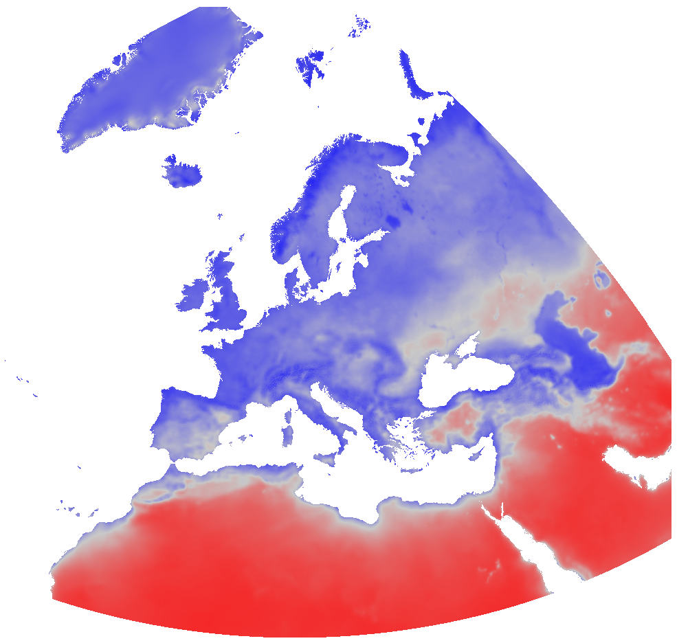
Overview: ERA5-Land is a reanalysis dataset providing a consistent view of the evolution of land variables over several decades at an enhanced resolution compared to ERA5. ERA5-Land has been produced by replaying the land component of the ECMWF ERA5 climate reanalysis. Reanalysis combines model data with observations from across the world into a globally complete and consistent dataset using the laws of physics. Reanalysis produces data that goes several decades back in time, providing an accurate description of the climate of the past. Processing steps: The original hourly ERA5-Land air temperature 2 m above ground and dewpoint temperature 2 m data has been spatially enhanced from 0.1 degree to 30 arc seconds (approx. 1000 m) spatial resolution by image fusion with CHELSA data (V1.2) (https://chelsa-climate.org/). For each day we used the corresponding monthly long-term average of CHELSA. The aim was to use the fine spatial detail of CHELSA and at the same time preserve the general regional pattern and fine temporal detail of ERA5-Land. The steps included aggregation and enhancement, specifically: 1. spatially aggregate CHELSA to the resolution of ERA5-Land 2. calculate difference of ERA5-Land - aggregated CHELSA 3. interpolate differences with a Gaussian filter to 30 arc seconds. 4. add the interpolated differences to CHELSA Subsequently, the temperature time series have been aggregated on a daily basis. From these, daily relative humidity has been calculated for the time period 01/2000 - 12/2023. Relative humidity (rh2m) has been calculated from air temperature 2 m above ground (Ta) and dewpoint temperature 2 m above ground (Td) using the formula for saturated water pressure from Wright (1997): maximum water pressure = 611.21 * exp(17.502 * Ta / (240.97 + Ta)) actual water pressure = 611.21 * exp(17.502 * Td / (240.97 + Td)) relative humidity = actual water pressure / maximum water pressure The resulting relative humidity has been aggregated to monthly averages. Resultant values have been converted to represent percent * 10, thus covering a theoretical range of [0, 1000]. The data have been reprojected to EU LAEA. File naming scheme (YYYY = year; MM = month): ERA5_land_rh2m_avg_monthly_YYYY_MM.tif Projection + EPSG code: EU LAEA (EPSG: 3035) Spatial extent: north: 6874000 south: -485000 west: 869000 east: 8712000 Spatial resolution: 1000 m Temporal resolution: Monthly Pixel values: Percent * 10 (scaled to Integer; example: value 738 = 73.8 %) Software used: GDAL 3.2.2 and GRASS GIS 8.0.0/8.3.2 Original ERA5-Land dataset license: https://apps.ecmwf.int/datasets/licences/copernicus/ CHELSA climatologies (V1.2): Data used: Karger D.N., Conrad, O., Böhner, J., Kawohl, T., Kreft, H., Soria-Auza, R.W., Zimmermann, N.E, Linder, H.P., Kessler, M. (2018): Data from: Climatologies at high resolution for the earth's land surface areas. Dryad digital repository. http://dx.doi.org/doi:10.5061/dryad.kd1d4 Original peer-reviewed publication: Karger, D.N., Conrad, O., Böhner, J., Kawohl, T., Kreft, H., Soria-Auza, R.W., Zimmermann, N.E., Linder, P., Kessler, M. (2017): Climatologies at high resolution for the Earth land surface areas. Scientific Data. 4 170122. https://doi.org/10.1038/sdata.2017.122 Processed by: mundialis GmbH & Co. KG, Germany (https://www.mundialis.de/) Reference: Wright, J.M. (1997): Federal meteorological handbook no. 3 (FCM-H3-1997). Office of Federal Coordinator for Meteorological Services and Supporting Research. Washington, DC Data is also available in Latitude-Longitude/WGS84 (EPSG: 4326) projection: https://data.mundialis.de/geonetwork/srv/eng/catalog.search#/metadata/b9ce7dba-4130-428d-96f0-9089d8b9f4a5 Acknowledgements: This study was partially funded by EU grant 874850 MOOD. The contents of this publication are the sole responsibility of the authors and don't necessarily reflect the views of the European Commission.

osm: Farmyard rasterized from OSM landuse polygons, first to 10m spatial resolution and after downsampled to 30m by spatial average.

122: Motorways and railways, including associated installations (stations, platforms, embankments, linear greenery narrower than 100 m). Minimum width for inclusion: 100 m. The general requirement of 100 m delineation accuracy is not sufficient in mapping 122. The tolerable shift in delineation is maximum 50 m. In delineating 122 a maximum 15-20% exaggeration of width is allowed, meaning that real width of the road including associated land should be at least 80 m to be included in CLC. In such cases the exaggerated width should be as close as possible to 100 m.