 Open Data Science Europe Metadata Catalog
Type of resources
Available actions
Topics
Keywords
Contact for the resource
Provided by
Years
Formats
Representation types
Update frequencies
status
Service types
Scale
Resolution
-

Regional model ICON-D2 The DWD's ICON-D2 model is a forecast model which is operated for the very-short range up to +27 hours (+45 hours for the 03 UTC run). Due to its fine mesh size, the ICON-D2 especially provides for improved forecasts of hazardous weather conditions, e.g. weather situations with high-level moisture convection (super and multi-cell thunderstorms, squall lines, mesoscale convective complexes) and weather events that are influenced by fine-scale topographic effects (ground fog, Föhn winds, intense downslope winds, flash floods). The model area of ICON-D2 covers the whole German territory, Benelux, Switzerland, Austria and parts of the other neighbouring countries at a horizontal resolution of 2.2 km. In the vertical, the model defines 65 atmosphere levels. The fairly short forecast periods make perfect sense because of the purpose of ICON-D2 (and its small model area). Based on model runs at 00, 06, 09, 12, 15, 18 and 21 UTC, ICON-D2 provides new 27-hour forecasts every 3 hours. The model run at 03 UTC even covers a forecast period of 45 hours. The ICON-D2 forecast data for each weather element are made available in standard packages at our free DWD Open Data Server, both on a rotated grid and on a regular grid. Regional ensemble forecast model ICON-D2 EPS The ensemble forecasting system ICON-D2 EPS is based on the DWD's numerical weather forecast model ICON-D2 and currently includes 20 ensemble members. All ensemble members are calculated at the same horizontal grid spacing as the operational configuration of ICON-D2 (2.2 km). Like ICON-D2, the ICON-D2 EPS ensemble system provides forecasts up to +27 hours for the same model area (up to +45 hours based on the 03 UTC run). For generating the ensemble members, some of the features of the forecasting system are changed. The method currently used to generate the ensemble members involves varying the - lateral boundary conditions - initial state - soil moisture - and model physics. For varying the lateral boundary conditions and the initial state, forecasts from various global models are used. The ICON-D2 EPS is provided on the DWD Open Data Server in the native triangular grid. Note: All previously COSMO-D2 based aviation weather products have been migrated to ICON-D2 on 10.02.2021. However, the familiar design of these products remains unchanged.
-
Overview: 243: Areas principally occupied with agriculture, interspersed with significantsemi-natural areas in a mosaic pattern. Traceability (lineage): This dataset was produced with a machine learning framework with several input datasets, specified in detail in Witjes et al., 2022 (in review, preprint available at https://doi.org/10.21203/rs.3.rs-561383/v3 ) Scientific methodology: The single-class probability layers were generated with a spatiotemporal ensemble machine learning framework detailed in Witjes et al., 2022 (in review, preprint available at https://doi.org/10.21203/rs.3.rs-561383/v3 ). The single-class uncertainty layers were calculated by taking the standard deviation of the three single-class probabilities predicted by the three components of the ensemble. The HCL (hard class) layers represents the class with the highest probability as predicted by the ensemble. Usability: The HCL layers have a decreasing average accuracy (weighted F1-score) at each subsequent level in the CLC hierarchy. These metrics are 0.83 at level 1 (5 classes):, 0.63 at level 2 (14 classes), and 0.49 at level 3 (43 classes). This means that the hard-class maps are more reliable when aggregating classes to a higher level in the hierarchy (e.g. 'Discontinuous Urban Fabric' and 'Continuous Urban Fabric' to 'Urban Fabric'). Some single-class probabilities may more closely represent actual patterns for some classes that were overshadowed by unequal sample point distributions. Users are encouraged to set their own thresholds when postprocessing these datasets to optimize the accuracy for their specific use case. Uncertainty quantification: Uncertainty is quantified by taking the standard deviation of the probabilities predicted by the three components of the spatiotemporal ensemble model. Data validation approaches: The LULC classification was validated through spatial 5-fold cross-validation as detailed in the accompanying publication. Completeness: The dataset has chunks of empty predictions in regions with complex coast lines (e.g. the Zeeland province in the Netherlands and the Mar da Palha bay area in Portugal). These are artifacts that will be avoided in subsequent versions of the LULC product. Consistency: The accuracy of the predictions was compared per year and per 30km*30km tile across europe to derive temporal and spatial consistency by calculating the standard deviation. The standard deviation of annual weighted F1-score was 0.135, while the standard deviation of weighted F1-score per tile was 0.150. This means the dataset is more consistent through time than through space: Predictions are notably less accurate along the Mediterrranean coast. The accompanying publication contains additional information and visualisations. Positional accuracy: The raster layers have a resolution of 30m, identical to that of the Landsat data cube used as input features for the machine learning framework that predicted it. Temporal accuracy: The dataset contains predictions and uncertainty layers for each year between 2000 and 2019. Thematic accuracy: The maps reproduce the Corine Land Cover classification system, a hierarchical legend that consists of 5 classes at the highest level, 14 classes at the second level, and 44 classes at the third level. Class 523: Oceans was omitted due to computational constraints.
-
Overview: 241: Cultivated land parcels with a mixed coverage of non-permanent (e.g. wheat) and permanentcrops (e.g. olive trees) Traceability (lineage): This dataset was produced with a machine learning framework with several input datasets, specified in detail in Witjes et al., 2022 (in review, preprint available at https://doi.org/10.21203/rs.3.rs-561383/v3 ) Scientific methodology: The single-class probability layers were generated with a spatiotemporal ensemble machine learning framework detailed in Witjes et al., 2022 (in review, preprint available at https://doi.org/10.21203/rs.3.rs-561383/v3 ). The single-class uncertainty layers were calculated by taking the standard deviation of the three single-class probabilities predicted by the three components of the ensemble. The HCL (hard class) layers represents the class with the highest probability as predicted by the ensemble. Usability: The HCL layers have a decreasing average accuracy (weighted F1-score) at each subsequent level in the CLC hierarchy. These metrics are 0.83 at level 1 (5 classes):, 0.63 at level 2 (14 classes), and 0.49 at level 3 (43 classes). This means that the hard-class maps are more reliable when aggregating classes to a higher level in the hierarchy (e.g. 'Discontinuous Urban Fabric' and 'Continuous Urban Fabric' to 'Urban Fabric'). Some single-class probabilities may more closely represent actual patterns for some classes that were overshadowed by unequal sample point distributions. Users are encouraged to set their own thresholds when postprocessing these datasets to optimize the accuracy for their specific use case. Uncertainty quantification: Uncertainty is quantified by taking the standard deviation of the probabilities predicted by the three components of the spatiotemporal ensemble model. Data validation approaches: The LULC classification was validated through spatial 5-fold cross-validation as detailed in the accompanying publication. Completeness: The dataset has chunks of empty predictions in regions with complex coast lines (e.g. the Zeeland province in the Netherlands and the Mar da Palha bay area in Portugal). These are artifacts that will be avoided in subsequent versions of the LULC product. Consistency: The accuracy of the predictions was compared per year and per 30km*30km tile across europe to derive temporal and spatial consistency by calculating the standard deviation. The standard deviation of annual weighted F1-score was 0.135, while the standard deviation of weighted F1-score per tile was 0.150. This means the dataset is more consistent through time than through space: Predictions are notably less accurate along the Mediterrranean coast. The accompanying publication contains additional information and visualisations. Positional accuracy: The raster layers have a resolution of 30m, identical to that of the Landsat data cube used as input features for the machine learning framework that predicted it. Temporal accuracy: The dataset contains predictions and uncertainty layers for each year between 2000 and 2019. Thematic accuracy: The maps reproduce the Corine Land Cover classification system, a hierarchical legend that consists of 5 classes at the highest level, 14 classes at the second level, and 44 classes at the third level. Class 523: Oceans was omitted due to computational constraints.
-
222: Cultivated parcels planted with fruit trees and shrubs, intended for fruit production, including nuts. The planting pattern can be by single or mixed fruit species, both in association with permanently grassy surfaces.
-
pm2.5: Number of pixels used in aggregating monthly PM2.5 maps.
-
Overview: Potential Natural Vegetation (PNV): potential probability of occurrence for the Pedunculate oak from 2018 to 2020 Traceability (lineage): This is an original dataset produced with a machine learning framework which used a combination of point datasets and raster datasets as inputs. Point dataset is a harmonized collection of tree occurrence data, comprising observations from National Forest Inventories (EU-Forest), GBIF and LUCAS. The complete dataset is available on Zenodo. Raster datasets used as input are: monthly time series air and surface temperature and precipitation from a reprocessed version of the Copernicus ERA5 dataset; long term averages of bioclimatic variables from CHELSA; elevation, slope and other elevation-derived metrics and long term monthly averages snow probability. For a more comprehensive list refer to Bonannella et al. (2022) (in review, preprint available at: https://doi.org/10.21203/rs.3.rs-1252972/v1). Scientific methodology: Probability and uncertainty maps were the output of a spatiotemporal ensemble machine learning framework based on stacked regularization. Three base models (random forest, gradient boosted trees and generalized linear models) were first trained on the input dataset and their predictions were used to train an additional model (logistic regression) which provided the final predictions. More details on the whole workflow are available in the listed publication. Usability: Probability maps are particularly useful when compared with existing products of potential distribution of species or when combined with maps of realized distribution: gaps in potential and realized distribution can be identified and used as information for future programs of tree planting or forest restoration. Uncertainty quantification: Uncertainty is quantified by taking the standard deviation of the probabilities predicted by the three components of the spatiotemporal ensemble model. Data validation approaches: Distribution maps were validated using a spatial 5-fold cross validation following the workflow detailed in the listed publication. Completeness: The raster files perfectly cover the entire Geo-harmonizer region as defined by the landmask raster dataset available here. Consistency: Areas which are outside of the calibration area of the point dataset (Iceland, Norway) usually have high uncertainty values. This is not only a problem of extrapolation but also of poor representation in the feature space available to the model of the conditions that are present in this countries. Positional accuracy: The rasters have a spatial resolution of 30m. Temporal accuracy: The maps cover the period 2018 - 2020 Thematic accuracy: Both probability and uncertainty maps contain values from 0 to 100: in the case of probability maps, they indicate the probability of occurrence of a single individual of the target species, while uncertainty maps indicate the standard deviation of the ensemble model.
-
421: Vegetated low-lying areas in the coastal zone, above the high-tide line, susceptible to flooding by seawater. Often in the process of being filled in by coastal mud and sand sediments, gradually being colonized by halophilic plants. Salt marshes are in most cases directly connected to intertidal areas and may successively develop from them in the long-term. Salt-pans for extraction of salt from salt water by evaporation, active or in process of abandonment. Sections of salt marsh exploited for the production of salt, clearly distinguishable from the rest of the marsh by their parcellation and embankment systems. Coastal zone under tidal influence between open sea and land, which is flooded by sea water regularly twice a day in a ca. 12 hours cycle. Area between the average lowest and highest sea water level at low tide and high tide. Generally non-vegetated expanses of mud, sand or rock lying between high and low water marks. The seaward boundary of intertidal flats may underlay constant change in geographical extent due to littoral morphodynamics. Range of water level between low tide and high tide may vary between decimeters and several meters in height.
-
Overview: Potential Natural Vegetation (PNV): potential probability of occurrence for the Turkey oak from 2018 to 2020 Traceability (lineage): This is an original dataset produced with a machine learning framework which used a combination of point datasets and raster datasets as inputs. Point dataset is a harmonized collection of tree occurrence data, comprising observations from National Forest Inventories (EU-Forest), GBIF and LUCAS. The complete dataset is available on Zenodo. Raster datasets used as input are: monthly time series air and surface temperature and precipitation from a reprocessed version of the Copernicus ERA5 dataset; long term averages of bioclimatic variables from CHELSA; elevation, slope and other elevation-derived metrics and long term monthly averages snow probability. For a more comprehensive list refer to Bonannella et al. (2022) (in review, preprint available at: https://doi.org/10.21203/rs.3.rs-1252972/v1). Scientific methodology: Probability and uncertainty maps were the output of a spatiotemporal ensemble machine learning framework based on stacked regularization. Three base models (random forest, gradient boosted trees and generalized linear models) were first trained on the input dataset and their predictions were used to train an additional model (logistic regression) which provided the final predictions. More details on the whole workflow are available in the listed publication. Usability: Probability maps are particularly useful when compared with existing products of potential distribution of species or when combined with maps of realized distribution: gaps in potential and realized distribution can be identified and used as information for future programs of tree planting or forest restoration. Uncertainty quantification: Uncertainty is quantified by taking the standard deviation of the probabilities predicted by the three components of the spatiotemporal ensemble model. Data validation approaches: Distribution maps were validated using a spatial 5-fold cross validation following the workflow detailed in the listed publication. Completeness: The raster files perfectly cover the entire Geo-harmonizer region as defined by the landmask raster dataset available here. Consistency: Areas which are outside of the calibration area of the point dataset (Iceland, Norway) usually have high uncertainty values. This is not only a problem of extrapolation but also of poor representation in the feature space available to the model of the conditions that are present in this countries. Positional accuracy: The rasters have a spatial resolution of 30m. Temporal accuracy: The maps cover the period 2018 - 2020 Thematic accuracy: Both probability and uncertainty maps contain values from 0 to 100: in the case of probability maps, they indicate the probability of occurrence of a single individual of the target species, while uncertainty maps indicate the standard deviation of the ensemble model.
-
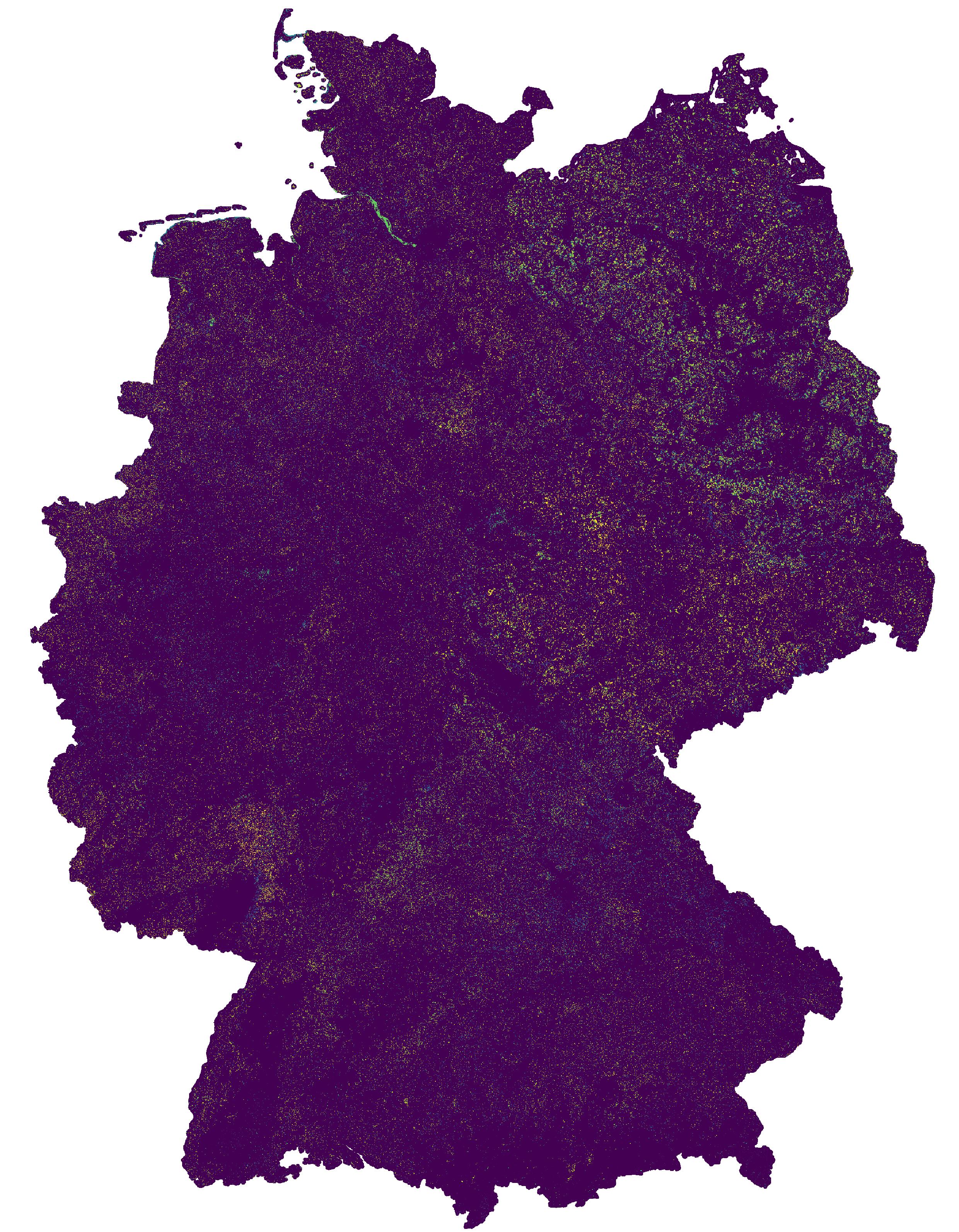
This change map was produced on the basis of a classification method developed in the project incora (Inwertsetzung von Copernicus-Daten für die Raumbeobachtung, mFUND Förderkennzeichen: 19F2079C) in cooperation with ILS (Institut für Landes- und Stadtentwicklungsforschung gGmbH) and BBSR (Bundesinstitut für Bau-, Stadt- und Raumforschung) funded by BMVI (Federal Ministry of Transport and Digital Infrastructure). The goal of incora is an analysis of settlement and infrastructure dynamics in Germany based on Copernicus Sentinel data. The map indicates land cover changes between the years 2019 and 2020. It is a difference map from two classifications based on Sentinel-2 MAJA data (MAJA L3A-WASP: https://geoservice.dlr.de/web/maps/sentinel2:l3a:wasp; DLR (2019): Sentinel-2 MSI - Level 2A (MAJA-Tiles)- Germany). More information on the two basis classifications can be found here: https://data.mundialis.de/geonetwork/srv/eng/catalog.search#/metadata/36512b46-f3aa-4aa4-8281-7584ec46c813 https://data.mundialis.de/geonetwork/srv/eng/catalog.search#/metadata/9246503f-6adf-460b-a31e-73a649182d07 To keep only significant changes in the change detection map, the following postprocessing steps are applied to the initial difference raster: - Modefilter (3x3) to eliminate isolated pixels and edge effects - Information gain in a 4x4 window compares class distribution within the window from the two timesteps. High values indicate that the class distribution in the window has changed, and thus a change is likely. Gain ranges from 0 to 1, all changes < 0.5 are omitted. - Change areas < 1ha are removed The resulting map has the following nomenclature: 0: No Change 1: Change from low vegetation to forest 2: Change from water to forest 3: Change from built-up to forest 4: Change from bare soil to forest 5: Change from agriculture to forest 6: Change from forest to low vegetation 7: Change from water to low vegetation 8: Change from built-up to low vegetation 9: Change from bare soil to low vegetation 10: Change from agriculture to low vegetation 11: Change from forest to water 12: Change from low vegetation to water 13: Change from built-up to water 14: Change from bare soil to water 15: Change from agriculture to water 16: Change from forest to built-up 17: Change from low vegetation to built-up 18: Change from water to built-up 19: Change from bare soil to built-up 20: Change from agriculture to built-up 21: Change from forest to bare soil 22: Change from low vegetation to bare soil 23: Change from water to bare soil 24: Change from built-up to bare soil 25: Change from agriculture to bare soil 26: Change from forest to agriculture 27: Change from low vegetation to agriculture 28: Change from water to agriculture 29: Change from built-up to agriculture 30: Change from bare soil to agriculture - Contains modified Copernicus Sentinel data (2019/2020), processed by mundialis Incora report with details on methods and results: pending
-
Overview: 244: Annual crops or grazing land under the wooded cover of forestry species. Traceability (lineage): This dataset was produced with a machine learning framework with several input datasets, specified in detail in Witjes et al., 2022 (in review, preprint available at https://doi.org/10.21203/rs.3.rs-561383/v3 ) Scientific methodology: The single-class probability layers were generated with a spatiotemporal ensemble machine learning framework detailed in Witjes et al., 2022 (in review, preprint available at https://doi.org/10.21203/rs.3.rs-561383/v3 ). The single-class uncertainty layers were calculated by taking the standard deviation of the three single-class probabilities predicted by the three components of the ensemble. The HCL (hard class) layers represents the class with the highest probability as predicted by the ensemble. Usability: The HCL layers have a decreasing average accuracy (weighted F1-score) at each subsequent level in the CLC hierarchy. These metrics are 0.83 at level 1 (5 classes):, 0.63 at level 2 (14 classes), and 0.49 at level 3 (43 classes). This means that the hard-class maps are more reliable when aggregating classes to a higher level in the hierarchy (e.g. 'Discontinuous Urban Fabric' and 'Continuous Urban Fabric' to 'Urban Fabric'). Some single-class probabilities may more closely represent actual patterns for some classes that were overshadowed by unequal sample point distributions. Users are encouraged to set their own thresholds when postprocessing these datasets to optimize the accuracy for their specific use case. Uncertainty quantification: Uncertainty is quantified by taking the standard deviation of the probabilities predicted by the three components of the spatiotemporal ensemble model. Data validation approaches: The LULC classification was validated through spatial 5-fold cross-validation as detailed in the accompanying publication. Completeness: The dataset has chunks of empty predictions in regions with complex coast lines (e.g. the Zeeland province in the Netherlands and the Mar da Palha bay area in Portugal). These are artifacts that will be avoided in subsequent versions of the LULC product. Consistency: The accuracy of the predictions was compared per year and per 30km*30km tile across europe to derive temporal and spatial consistency by calculating the standard deviation. The standard deviation of annual weighted F1-score was 0.135, while the standard deviation of weighted F1-score per tile was 0.150. This means the dataset is more consistent through time than through space: Predictions are notably less accurate along the Mediterrranean coast. The accompanying publication contains additional information and visualisations. Positional accuracy: The raster layers have a resolution of 30m, identical to that of the Landsat data cube used as input features for the machine learning framework that predicted it. Temporal accuracy: The dataset contains predictions and uncertainty layers for each year between 2000 and 2019. Thematic accuracy: The maps reproduce the Corine Land Cover classification system, a hierarchical legend that consists of 5 classes at the highest level, 14 classes at the second level, and 44 classes at the third level. Class 523: Oceans was omitted due to computational constraints.