Regional model ICON-D2 The DWD's ICON-D2 model is a forecast model which is operated for the very-short range up to +27 hours (+45 hours for the 03 UTC run). Due to its fine mesh size, the ICON-D2 especially provides for improved forecasts of hazardous weather conditions, e.g. weather situations with high-level moisture convection (super and multi-cell thunderstorms, squall lines, mesoscale convective complexes) and weather events that are influenced by fine-scale topographic effects (ground fog, Föhn winds, intense downslope winds, flash floods). The model area of ICON-D2 covers the whole German territory, Benelux, Switzerland, Austria and parts of the other neighbouring countries at a horizontal resolution of 2.2 km. In the vertical, the model defines 65 atmosphere levels. The fairly short forecast periods make perfect sense because of the purpose of ICON-D2 (and its small model area). Based on model runs at 00, 06, 09, 12, 15, 18 and 21 UTC, ICON-D2 provides new 27-hour forecasts every 3 hours. The model run at 03 UTC even covers a forecast period of 45 hours. The ICON-D2 forecast data for each weather element are made available in standard packages at our free DWD Open Data Server, both on a rotated grid and on a regular grid. Regional ensemble forecast model ICON-D2 EPS The ensemble forecasting system ICON-D2 EPS is based on the DWD's numerical weather forecast model ICON-D2 and currently includes 20 ensemble members. All ensemble members are calculated at the same horizontal grid spacing as the operational configuration of ICON-D2 (2.2 km). Like ICON-D2, the ICON-D2 EPS ensemble system provides forecasts up to +27 hours for the same model area (up to +45 hours based on the 03 UTC run). For generating the ensemble members, some of the features of the forecasting system are changed. The method currently used to generate the ensemble members involves varying the - lateral boundary conditions - initial state - soil moisture - and model physics. For varying the lateral boundary conditions and the initial state, forecasts from various global models are used. The ICON-D2 EPS is provided on the DWD Open Data Server in the native triangular grid. Note: All previously COSMO-D2 based aviation weather products have been migrated to ICON-D2 on 10.02.2021. However, the familiar design of these products remains unchanged.

Areas planted with vines, vineyard parcels covering >50% and determining the land use of the area.

The Land Cover Map of Europe 2017 is a product resulting from the Phase 2 of the S2GLC project. The final map has been produced on the CREODIAS platform with algorithms and software developed by CBK PAN. Classification of over 15 000 Sentinel-2 images required high level of automation that was assured by the developed software. The legend of the resulting Land Cover Map of Europe 2017 consists of 13 land cover classes. The pixel size of the map equals 10 m, which corresponds to the highest spatial resolution of Sentinel-2 imagery. Its overall accuracy was estimated to be at the level of 86% using approximately 52 000 validation samples distributed across Europe. Related publication: https://doi.org/10.3390/rs12213523

Overview: 211: Slope of non-irrigated arable land derived by OLS regression over the probabilities values (2000—2019). The std. error of the model was considered as uncertainty. Traceability (lineage): This dataset was produced with a machine learning framework with several input datasets, specified in detail in Witjes et al., 2022 (in review, preprint available at https://doi.org/10.21203/rs.3.rs-561383/v3 ) Scientific methodology: The single-class probability layers were generated with a spatiotemporal ensemble machine learning framework detailed in Witjes et al., 2022 (in review, preprint available at https://doi.org/10.21203/rs.3.rs-561383/v3 ). The single-class uncertainty layers were calculated by taking the standard deviation of the three single-class probabilities predicted by the three components of the ensemble. The HCL (hard class) layers represents the class with the highest probability as predicted by the ensemble. Usability: The HCL layers have a decreasing average accuracy (weighted F1-score) at each subsequent level in the CLC hierarchy. These metrics are 0.83 at level 1 (5 classes):, 0.63 at level 2 (14 classes), and 0.49 at level 3 (43 classes). This means that the hard-class maps are more reliable when aggregating classes to a higher level in the hierarchy (e.g. 'Discontinuous Urban Fabric' and 'Continuous Urban Fabric' to 'Urban Fabric'). Some single-class probabilities may more closely represent actual patterns for some classes that were overshadowed by unequal sample point distributions. Users are encouraged to set their own thresholds when postprocessing these datasets to optimize the accuracy for their specific use case. Uncertainty quantification: Uncertainty is quantified by taking the standard deviation of the probabilities predicted by the three components of the spatiotemporal ensemble model. Data validation approaches: The LULC classification was validated through spatial 5-fold cross-validation as detailed in the accompanying publication. Completeness: The dataset has chunks of empty predictions in regions with complex coast lines (e.g. the Zeeland province in the Netherlands and the Mar da Palha bay area in Portugal). These are artifacts that will be avoided in subsequent versions of the LULC product. Consistency: The accuracy of the predictions was compared per year and per 30km*30km tile across europe to derive temporal and spatial consistency by calculating the standard deviation. The standard deviation of annual weighted F1-score was 0.135, while the standard deviation of weighted F1-score per tile was 0.150. This means the dataset is more consistent through time than through space: Predictions are notably less accurate along the Mediterrranean coast. The accompanying publication contains additional information and visualisations. Positional accuracy: The raster layers have a resolution of 30m, identical to that of the Landsat data cube used as input features for the machine learning framework that predicted it. Temporal accuracy: The dataset contains predictions and uncertainty layers for each year between 2000 and 2019. Thematic accuracy: The maps reproduce the Corine Land Cover classification system, a hierarchical legend that consists of 5 classes at the highest level, 14 classes at the second level, and 44 classes at the third level. Class 523: Oceans was omitted due to computational constraints.

The Land Cover Map of Europe 2017 is a product resulting from the Phase 2 of the S2GLC project. The final map has been produced on the CREODIAS platform with algorithms and software developed by CBK PAN. Classification of over 15 000 Sentinel-2 images required high level of automation that was assured by the developed software. The legend of the resulting Land Cover Map of Europe 2017 consists of 13 land cover classes. The pixel size of the map equals 10 m, which corresponds to the highest spatial resolution of Sentinel-2 imagery. Its overall accuracy was estimated to be at the level of 86% using approximately 52 000 validation samples distributed across Europe. Related publication: https://doi.org/10.3390/rs12213523

osm: Farmland rasterized from OSM landuse polygons, first to 10m spatial resolution and after downsampled to 30m by spatial average.

The Land Processes Distributed Active Archive Center (LP DAAC) is responsible for the archive and distribution of NASA Making Earth System Data Records for Use in Research Environments (MEaSUREs) Digital Elevation Model (DEM) version 1 (NASADEM_SC) dataset, which provides global slope and curvature elevation data at 1 arc second spacing. NASADEM data products were derived from original telemetry data from the Shuttle Radar Topography Mission (SRTM), a collaboration between NASA and the National Geospatial-Intelligence Agency (NGA), as well as participation from the German and Italian space agencies. SRTM’s primary focus was to generate a near-global DEM of the Earth using radar interferometry. It was a primary component of the payload on space shuttle Endeavour during its STS-99 mission, which was launched on February 11, 2000, and flew for 11 days. In addition to Terra Advanced Spaceborne Thermal and Reflection Radiometer (ASTER) Global Digital Elevation Model (GDEM) Version 3 data, NASADEM also relied on Ice, Cloud, and Land Elevation Satellite (ICESat) Geoscience Laser Altimeter System (GLAS) ground control points of its lidar shots to improve surface elevation measurements that led to improved geolocation accuracy. Other reprocessing improvements include the conversion to geoid reference and the use of GDEMs and Advanced Land Observing Satellite Panchromatic Remote-sensing instrument for Stereo Mapping (PRISM) AW3D30 DEM, and interpolation for void filling. NASADEM are distributed in 1° by 1° tiles and consist of all land between 60° N and 56° S latitude. This accounts for about 80% of Earth’s total landmass. NASADEM_SC data product layers include slope, aspect angle, profile curvature, plan curvature, and an updated SRTM water body dataset (water mask). A low-resolution browse image showing slope is also available for each NASADEM_SC granule.

122: Motorways and railways, including associated installations (stations, platforms, embankments, linear greenery narrower than 100 m). Minimum width for inclusion: 100 m. The general requirement of 100 m delineation accuracy is not sufficient in mapping 122. The tolerable shift in delineation is maximum 50 m. In delineating 122 a maximum 15-20% exaggeration of width is allowed, meaning that real width of the road including associated land should be at least 80 m to be included in CLC. In such cases the exaggerated width should be as close as possible to 100 m.

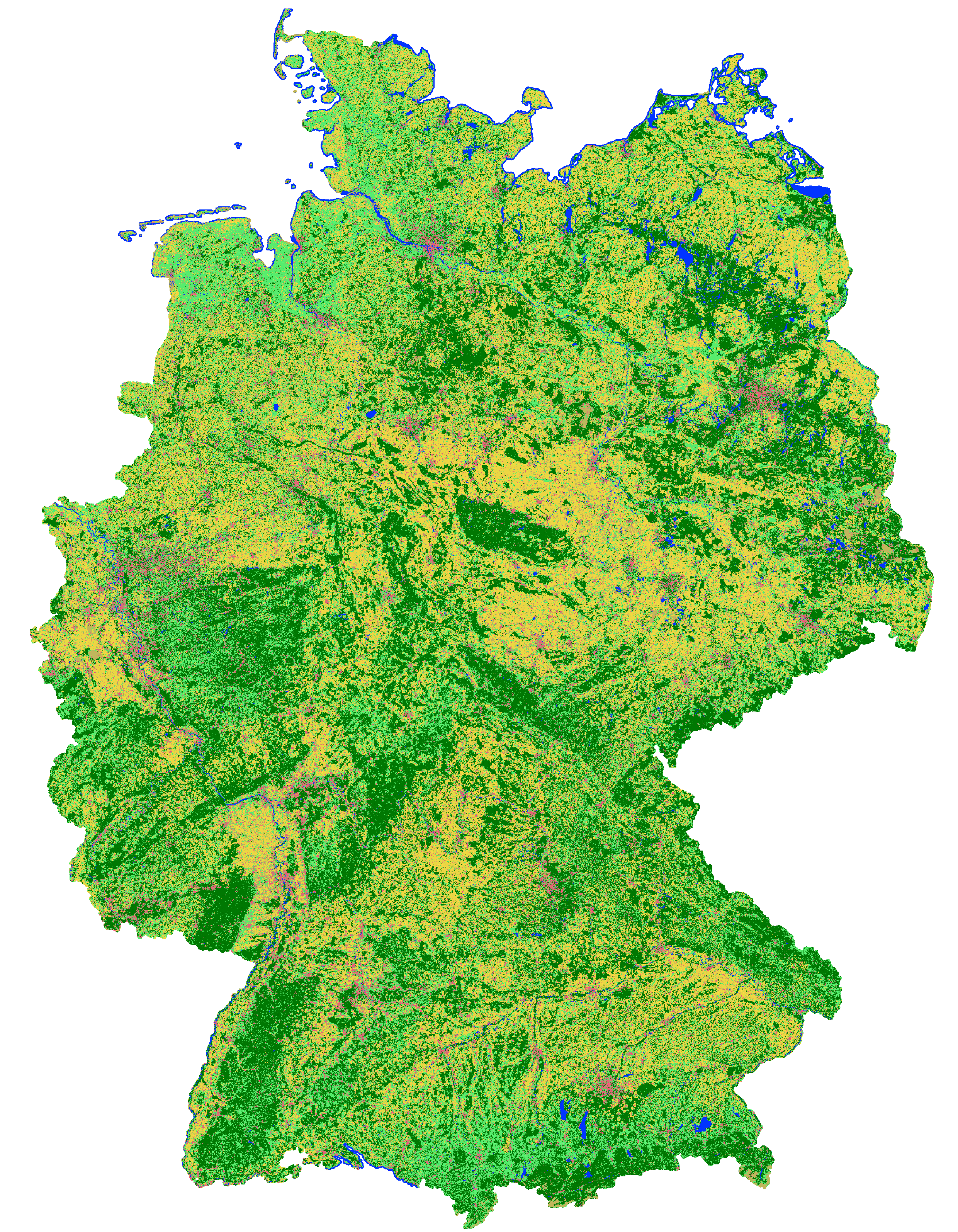
This landcover map was produced with a classification method developed in the project incora (Inwertsetzung von Copernicus-Daten für die Raumbeobachtung, mFUND Förderkennzeichen: 19F2079C) in cooperation with ILS (Institut für Landes- und Stadtentwicklungsforschung gGmbH) and BBSR (Bundesinstitut für Bau-, Stadt- und Raumforschung) funded by BMVI (Federal Ministry of Transport and Digital Infrastructure). The goal of incora is an analysis of settlement and infrastructure dynamics in Germany based on Copernicus Sentinel data. This classification is based on a time-series of monthly averaged, atmospherically corrected Sentinel-2 tiles (MAJA L3A-WASP: https://geoservice.dlr.de/web/maps/sentinel2:l3a:wasp; DLR (2019): Sentinel-2 MSI - Level 2A (MAJA-Tiles)- Germany). It consists of the following landcover classes: 10: forest 20: low vegetation 30: water 40: built-up 50: bare soil 60: agriculture Potential training and validation areas were automatically extracted using spectral indices and their temporal variability from the Sentinel-2 data itself as well as the following auxiliary datasets: - OpenStreetMap (Map data copyrighted OpenStreetMap contributors and available from htttps://www.openstreetmap.org) - Copernicus HRL Imperviousness Status Map 2018 (© European Union, Copernicus Land Monitoring Service 2018, European Environment Agency (EEA)) - S2GLC Land Cover Map of Europe 2017 (Malinowski et al. 2020: Automated Production of Land Cover/Use Map of Europe Based on Sentinel-2 Imagery. Remote Sens. 2020, 12(21), 3523; https://doi.org/10.3390/rs12213523) - Germany NUTS administrative areas 1:250000 (© GeoBasis-DE / BKG 2020 / dl-de/by-2-0 / https://gdz.bkg.bund.de/index.php/default/nuts-gebiete-1-250-000-stand-31-12-nuts250-31-12.html) - Contains modified Copernicus Sentinel data (2020), processed by mundialis Processing was performed for blocks of federal states and individual maps were mosaicked afterwards. For each class 100,000 pixels from the potential training areas were extracted as training data. An exemplary validation of the classification results was perfomed for the federal state of North Rhine-Westphalia as its open data policy allows for direct access to official data to be used as reference. Rules to convert relevant ATKIS Basis-DLM object classes to the incora nomenclature were defined. Subsequently, 5.000 reference points were randomly sampled and their classification in each case visually examined and, if necessary, revised to obtain a robust reference data set. The comparison of this reference data set with the incora classification yielded the following results: overall accurary: 88.4% class: user's accuracy / producer's accurary (number of reference points n) forest: 95.0% / 93.8% (1410) low vegetation: 73.4% / 86.5% (844) water: 98.5% / 92.8% (69) built-up: 98.9% / 95.8% (983) bare soil: 23.9% / 82.9% (41) agriculture: 94.6% / 83.2% (1653) Incora report with details on methods and results: pending