 Open Data Science Europe Metadata Catalog
Geoscientific information
Type of resources
Available actions
Topics
Keywords
Contact for the resource
Provided by
Years
Formats
Representation types
Update frequencies
status
Scale
Resolution
-

To meet the demand for statistics at a local level, Eurostat maintains a system of Local Administrative Units (LAUs) compatible with NUTS. These LAUs are the building blocks of the NUTS, and comprise the municipalities and communes of the European Union. The LAUs are: - administrative for reasons such as the availability of data and policy implementation capacity; - a subdivision of the NUTS 3 regions covering the whole economic territory of the Member States; - appropriate for the implementation of local level typologies included in TERCET, namely the coastal area and DEGURBA classification. Since there are frequent changes to the LAUs, Eurostat publishes an updated list towards the end of each year. The LAUs are currently available from 2011 onwards. The NUTS regulation makes provision for EU Member States to send the lists of their LAUs to Eurostat. If available, Eurostat receives additionally basic administrative data by means of the annual LAU lists, namely total population and total area for each LAU.
-

Overview: The Essential Climate Variables for assessment of climate variability from 1979 to present dataset contains a selection of climatologies, monthly anomalies and monthly mean fields of Essential Climate Variables (ECVs) suitable for monitoring and assessment of climate variability and change. Selection criteria are based on accuracy and temporal consistency on monthly to decadal time scales. The ECV data products in this set have been estimated from climate reanalyses ERA-Interim and ERA5, and, depending on the source, may have been adjusted to account for biases and other known deficiencies. Data sources and adjustment methods used are described in the Product User Guide, as are various particulars such as the baseline periods used to calculate monthly climatologies and the corresponding anomalies. Surface air relative humidity: The ratio of the partial pressure of water vapour to the equilibrium vapour pressure of water at the same temperature near the surface. Spatial resolution: 0:15:00 (0.25°) Temporal resolution: monthly Temporal extent: 1979 - present Data unit: percent * 10 Data type: UInt8 CRS as EPSG: EPSG:4326 Processing time delay: one month
-
Harmonized tree species occurrence points (field observations) for Europe is a harmonized collection of existing data from GBIF, the EU-Forest project and the LUCAS survey. It has about 3 million observations and is supplemented by variables (e.g. location accuracy, land cover type, canopy height, etc.) which enable precise filtering for specific user applications. The data can be obtained from: https://doi.org/10.5281/zenodo.4061816
-

Base epoch 2015 from the Collection 3 of annual, global 100m land cover maps. Other available (consolidated) epochs: 2016 2017 2018 2019 Produced by the global component of the Copernicus Land Service, derived from PROBA-V satellite observations and ancillary datasets. The maps include: - a main discrete classification with 23 classes aligned with UN-FAO's Land Cover Classification System, - a set of versatile cover fractions: percentage (%) of ground cover for the 10 main classes - - a forest type layer quality layers on input data density Online map viewer: https://lcviewer.vito.be
-
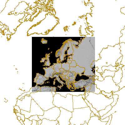
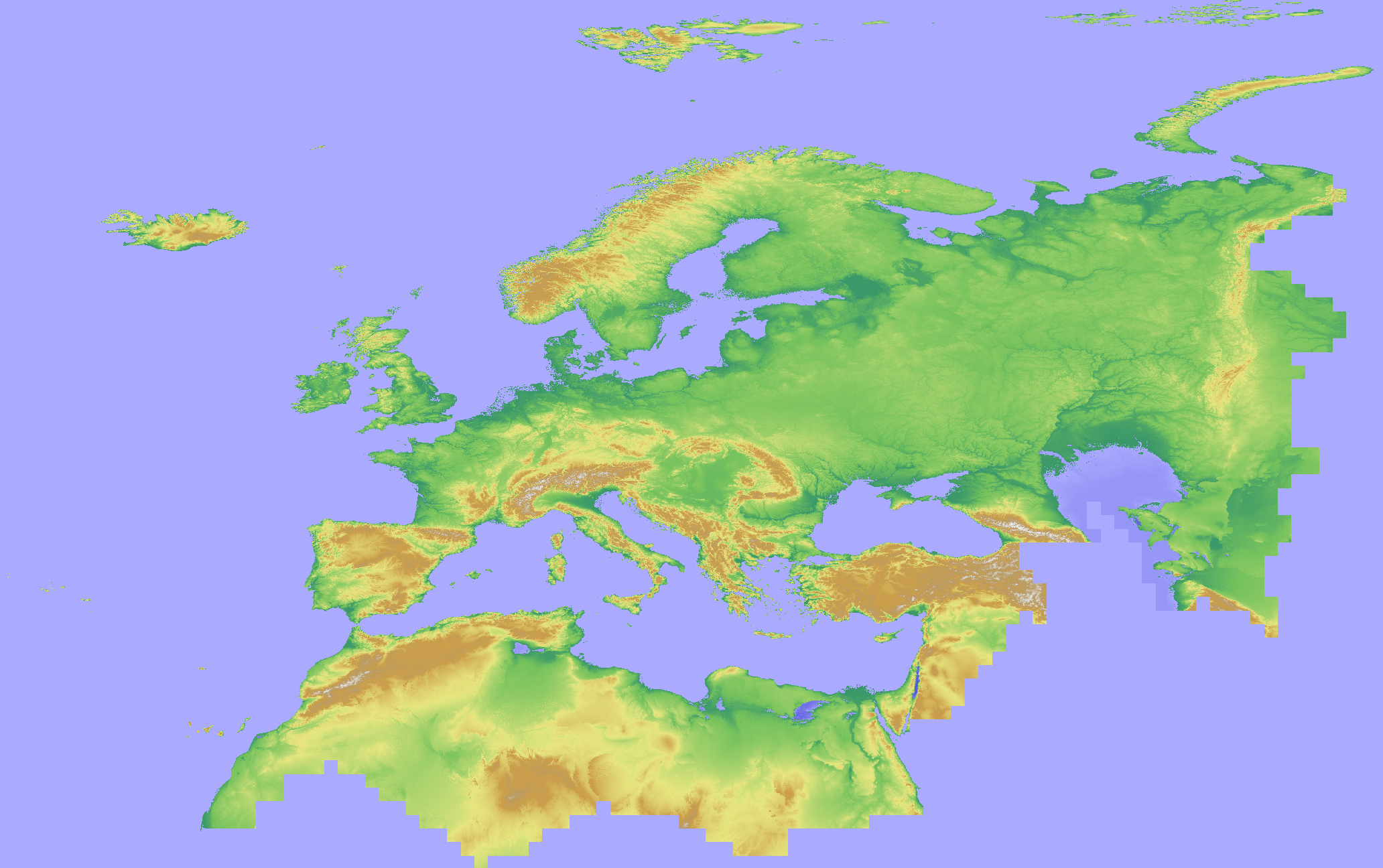
This is a cropped DTM version (with Frame2c) for providing topographic backgrouds on EEA maps. This is a hillshade of global digital elevation model (DEM) with a horizontal grid spacing of 30 arc seconds (approximately 1 kilometer).
-
The Copernicus DEM is a Digital Surface Model (DSM) which represents the surface of the Earth including buildings, infrastructure and vegetation. The original GLO-30 provides worldwide coverage at 30 meters (refers to 10 arc seconds). Note that ocean areas do not have tiles, there one can assume height values equal to zero. Data is provided as Cloud Optimized GeoTIFFs. Note that the vertical unit for measurement of elevation height is meters. The Copernicus DEM for Europe at 30 meter resolution (EU-LAEA projection) in COG format has been derived from the Copernicus DEM GLO-30, mirrored on Open Data on AWS, dataset managed by Sinergise (https://registry.opendata.aws/copernicus-dem/). Processing steps: The original Copernicus GLO-30 DEM contains a relevant percentage of tiles with non-square pixels. We created a mosaic map in https://gdal.org/drivers/raster/vrt.html format and defined within the VRT file the rule to apply cubic resampling while reading the data, i.e. importing them into GRASS GIS for further processing. We chose cubic instead of bilinear resampling since the height-width ratio of non-square pixels is up to 1:5. Hence, artefacts between adjacent tiles in rugged terrain could be minimized: gdalbuildvrt -input_file_list list_geotiffs_MOOD.csv -r cubic -tr 0.000277777777777778 0.000277777777777778 Copernicus_DSM_30m_MOOD.vrt In order to reproject the data to EU-LAEA projection, bilinear resampling was performed in GRASS GIS (using r.proj) and the pixel values were scaled with 1000 (storing the pixels as Integer values) for data volume reduction. In addition, a hillshade raster map was derived from the resampled elevation map (using r.relief, GRASS GIS). Eventually, we exported the elevation and hillshade raster maps in Cloud Optimized GeoTIFF (COG) format, along with SLD and QML style files. Note that GLO-30 Public provides limited coverage at 30 meters because a small subset of tiles covering specific countries are not yet released to the public by the Copernicus Programme. Note that ocean areas do not have tiles, there one can assume height values equal to zero. Data is provided as Cloud Optimized GeoTIFFs.
-

This global accessibility map enumerates land-based travel time to the nearest densely-populated area for all areas between 85 degrees north and 60 degrees south for a nominal year 2015. Densely-populated areas are defined as contiguous areas with 1,500 or more inhabitants per square kilometer or a majority of built-up land cover types coincident with a population centre of at least 50,000 inhabitants. This map was produced through a collaboration between the University of Oxford Malaria Atlas Project (MAP), Google, the European Union Joint Research Centre (JRC), and the University of Twente, Netherlands. The underlying datasets used to produce the map, include roads (comprising the first ever global-scale use of Open Street Map and Google roads datasets), railways, rivers, lakes, oceans, topographic conditions (slope and elevation), landcover types, and national borders. These datasets were each allocated a speed or speeds of travel in terms of time to cross each pixel of that type. The datasets were then combined to produce a “friction surface”, a map where every pixel is allocated a nominal overall speed of travel based on the types occurring within that pixel. Least-cost-path algorithms (running in Google Earth Engine and, for high-latitude areas, in R) were used in conjunction with this friction surface to calculate the time of travel from all locations to the nearest city (by travel time). Cities were determined using the high-density-cover product created by the Global Human Settlement Project. Each pixel in the resultant accessibility map thus represents the modeled shortest time from that location to a city. Full Citation D.J. Weiss, A. Nelson, H.S. Gibson, W. Temperley, S. Peedell, A. Lieber, M. Hancher, E. Poyart, S. Belchior, N. Fullman, B. Mappin, U. Dalrymple, J. Rozier, T.C.D. Lucas, R.E. Howes, L.S. Tusting, S.Y. Kang, E. Cameron, D. Bisanzio, K.E. Battle, S. Bhatt, and P.W. Gething. A global map of travel time to cities to assess inequalities in accessibility in 2015. (2018). Nature. doi:10.1038/nature25181.
-

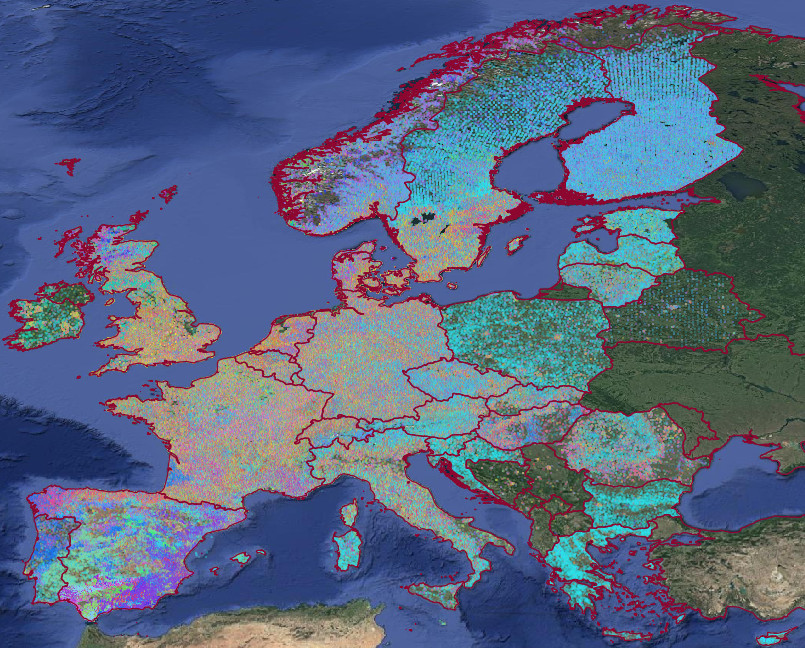
The Land Cover Map of Europe 2017 is a product resulting from the Phase 2 of the S2GLC project. The final map has been produced on the CREODIAS platform with algorithms and software developed by CBK PAN. Classification of over 15 000 Sentinel-2 images required high level of automation that was assured by the developed software. The legend of the resulting Land Cover Map of Europe 2017 consists of 13 land cover classes. The pixel size of the map equals 10 m, which corresponds to the highest spatial resolution of Sentinel-2 imagery. Its overall accuracy was estimated to be at the level of 86% using approximately 52 000 validation samples distributed across Europe. Related publication: https://doi.org/10.3390/rs12213523
-
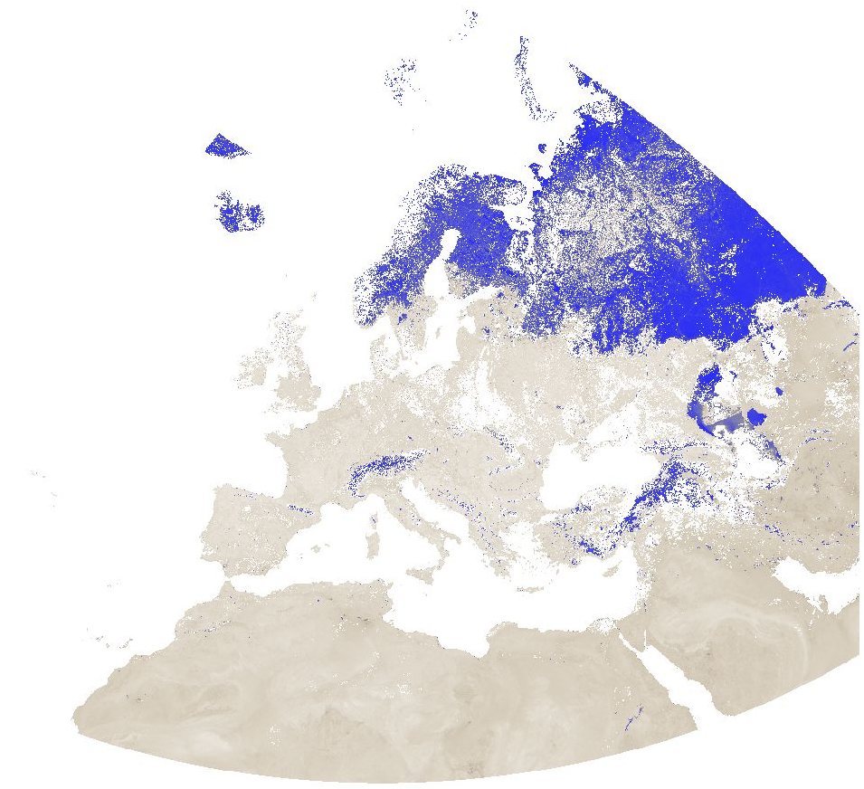
Modified Normalized Difference Water Index (MNDWI) from MODIS data for Europe at 1 km resolution. Source data: - MODIS/Terra Surface Reflectance 8-Day L3 Global 500 m SIN Grid (MOD09A1 v006): https://lpdaac.usgs.gov/products/mod09a1v006/ The corresponding MODIS/Aqua product (MYD09A1 v006) could not be used due to the fact that the Aqua satellite has a number of broken detectors resulting in unreliable data for band 6 (SWIR) measurements. The Moderate Resolution Imaging Spectroradiometer (MODIS) Terra MOD09A1 Version 6 product provides an estimate of the surface spectral reflectance of Terra MODIS Bands 1 through 7 corrected for atmospheric conditions such as gasses, aerosols, and Rayleigh scattering. Along with the seven 500 meter (m) reflectance bands are two quality layers and four observation bands. For each pixel, a value is selected from all the acquisitions within the 8-day composite period. The criteria for the pixel choice include cloud and solar zenith. When several acquisitions meet the criteria the pixel with the minimum channel 3 (blue) value is used. For the time periods October 2016 - March 2017 and August 2020 - April 2021, the original data has been reprojected to ETRS89-extended / LAEA Europe and aggregated to a 1 km grid. The temporal resolution is 8 days. Bad quality pixels (cloud, cloud shadow, dead detector, solar zenith angle too large, etc.) have been masked using the provided quality assurance (QA) layers and appear as "no data". File naming: productCode.acquisitionDate[A (YYYYDDD)]_mosaic_spatialResolution_frequency_VI.tif example: MOD09A1.A2016353_mosaic_1000m_8_days_MNDWI.tif The date is Year and Day of Year. Values are MNDWI * 10000. Example: Value -5099 = -0.5099
-
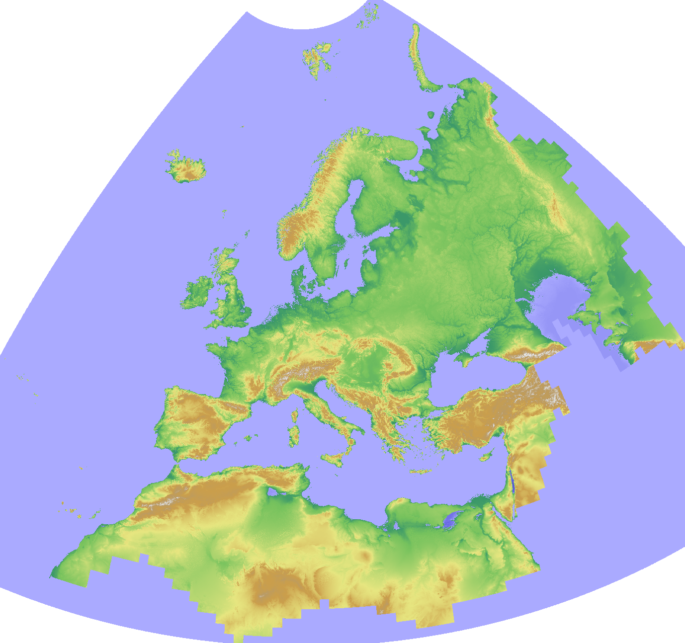
Here we provide a mosaic of the Copernicus DEM 30m for Europe and the corresponding hillshade derived from the GLO-30 public instance of the Copernicus DEM. The CRS is the same as the original Copernicus DEM CRS: EPSG:4326. Note that GLO-30 Public provides limited coverage at 30 meters because a small subset of tiles covering specific countries are not yet released to the public by the Copernicus Programme. Note that ocean areas do not have tiles, there one can assume height values equal to zero. Data is provided as Cloud Optimized GeoTIFFs. The Copernicus DEM is a Digital Surface Model (DSM) which represents the surface of the Earth including buildings, infrastructure and vegetation. The original GLO-30 provides worldwide coverage at 30 meters (refers to 10 arc seconds). Note that ocean areas do not have tiles, there one can assume height values equal to zero. Data is provided as Cloud Optimized GeoTIFFs. Note that the vertical unit for measurement of elevation height is meters. The Copernicus DEM for Europe at 30 m in COG format has been derived from the Copernicus DEM GLO-30, mirrored on Open Data on AWS, dataset managed by Sinergise (https://registry.opendata.aws/copernicus-dem/). Processing steps: The original Copernicus GLO-30 DEM contains a relevant percentage of tiles with non-square pixels. We created a mosaic map in https://gdal.org/drivers/raster/vrt.html format and defined within the VRT file the rule to apply cubic resampling while reading the data, i.e. importing them into GRASS GIS for further processing. We chose cubic instead of bilinear resampling since the height-width ratio of non-square pixels is up to 1:5. Hence, artefacts between adjacent tiles in rugged terrain could be minimized: gdalbuildvrt -input_file_list list_geotiffs_MOOD.csv -r cubic -tr 0.000277777777777778 0.000277777777777778 Copernicus_DSM_30m_MOOD.vrt The pixel values were scaled with 1000 (storing the pixels as integer values) for data volume reduction. In addition, a hillshade raster map was derived from the resampled elevation map (using r.relief, GRASS GIS). Eventually, we exported the elevation and hillshade raster maps in Cloud Optimized GeoTIFF (COG) format, along with SLD and QML style files.